Rate Limiting Techniques

13 min readFeb 19, 2021

Rate limiting is one of the most discussed topics related to protecting your APIs and services from excessive use either from bad actors trying to deliberately abuse the service or buggy code. Several people and companies have shared various approaches to implementing rate-limiting in applications, and there are several products that provide out-of-the-box support for rate limiting.

Rate limiting can either be global or on a per-client basis. The client here can refer to any user of a service. The client can be:

An actual user of the service (identified by some UserId or ClientId or DeviceId)
IP address
An internal service (identified by some ServiceId)

In this post, I tried to consolidate these techniques in one place and explain the pros and cons of different approaches.

Broadly, rate limiting can be implemented using one of the two approaches:

In-App

The application code (usually a request filter for HTTP requests) keeps track of the usage for various clients, typically using an external database or cache, and applies the limits when usage exceeds the quota.

The external datastore is required because usually there are multiple instances of a service running, and they need to share state to implement service-wide rate limiting. Redis is usually a good choice and is used widely for this use case.

Using a proxy

The second approach is to use a reverse proxy in front of the service instances.

Most popular proxies (Nginx, HAProxy, API Gateways, Envoy, etc.) come with rate-limiting functionality out of the box (However, it becomes tricky when there are multiple instances of the proxy itself).

We’ll discuss each of these approaches in detail below.

In-App Rate Limiting (Using Redis)

We’ll first discuss the in-app techniques for rate limiting. We’ll be using Redis as the database for our examples.

Fixed Window Counters

This is probably the simplest technique for implementing rate limiting. We define fixed-size time windows corresponding to our rate limit definition and count the number of client requests in those time windows. If the number of requests in any time window exceeds the defined quota, we block further requests from that client for the remainder of that window. Clients will have to wait till the start of the next window to make a successful request.

Suppose our rate limit is 3 requests/minute. When a request from a client (say with client ID = 12345) arrives, we do the following:

Get the current window start time. Since the time window is 1 minute, get the start of the current minute. For example, if the current time is 21/04/2020 10:00:23, then-current window start time is 21/04/2020 10:00:00.
Create a key in Redis which is a combination of the client ID and current window start time e.g. 12345_21042020_10:00:00 with value 1. If the key already exists, increment and get its value. If the value is greater than the number of allowed requests, block the request. Otherwise, let it in.

We can also use the Unix epoch timestamp. For example, the epoch corresponding to 21/04/2020 10:00:00 is 1587463200. Hence, the key in Redis will be 12345_1587463200.

Let’s see an example of a fixed window counter.

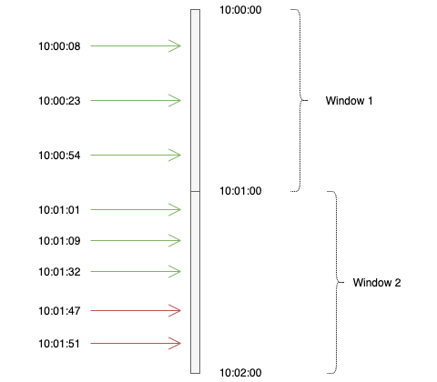
In this example, from the top, requests 1–3 belong to window 1, hence tracked against the same key in Redis (e.g. 12345_21042020_10:00:00 or 12345_1587463200 using epoch). Since there are only 3 requests in this window, no request is blocked.

Requests 4–8 belong to window 2 and will be tracked against the same key. After the first 3 requests have been allowed, the next 2 requests will be blocked as they exceed the defined quota.

Advantages

Simplicity
It can be used by multiple instances of a service since increment-and-get operation in Redis is atomic, so there will be no race conditions
Memory usage is low. It needs only one key per user per time window. Also, we can set the expiry of each key to be equal to (or slightly more than) the rate-limit window (1 minute in this case) so that at any time, the number of keys is equal to the number of active users.

Disadvantages

It can be a bit lenient i.e., it can allow more requests than intended by rate-limiting. For example, if our rate limit per user is 100 requests/min. A user can send 100 requests at 10:00:59 and another 100 requests at 10:01:01. This behavior is allowed by this algorithm. User is essentially able to send 200 requests in a span of 2 seconds, which violates the rate-limiting. However, depending on your use case, it may or may not be a problem.

Sliding Window Counters

To overcome the disadvantage of the fixed window approach, we can break the rate-limit window into smaller windows and track counters across those smaller windows. For example, in this case, instead of maintaining counters across a one-minute window, we can use one-second windows (so 60 sub-windows for a minute interval). To check whether to reject, we need to take a sum of counters of all previous 60 sub-windows from the current time. This essentially becomes a rolling window mechanism.

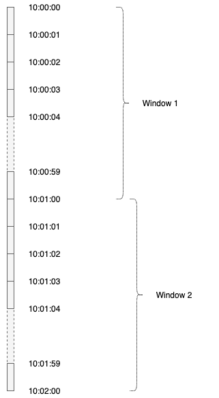
A new Redis key will be created for each 1-second sub-window, which will count all requests in that second. If a request arrives between 10:01:34 and 10:01:35, we take the sum of the value for keys 10:00:35, 10:00:36…up to 10:01:34.

Similarly, we can split a second window into X millisecond windows and so on.

We can have two approaches for storing the sub-windows:

Separate key for each sub-window (i.e. UserID_SubWindowEpoch). This is simple, and expiration is easy but will use more memory, and fetching (sum of all subwindows) is less efficient.
Keep only one key for a user and store sub-windows and counters in a hash. This is more memory-efficient (if hash has <100 keys). Each insert/update in the hash can extend the expiry of the parent hash key (since we can not have expiry for individual keys in the hash). If we don’t get requests from a user for some time, the entire hash will expire, and a new one will be created for the next request. This keeps overall memory low. However, if we keep getting requests from a user regularly, the hash will keep on growing, and we need to manually delete older keys from the hash. This approach is used by Figma.

Sliding Window Log

This approach uses Redis sorted sets and is described here in great detail. We basically keep a Redis sorted set for each user. Both value and score of the sorted set is the timestamp. For each request (assuming 1 min rate-limiting window):

Remove elements from the set which are older than 1 min using ZREMRANGEBYSCORE. This leaves only elements (requests) that occurred in the last 1 minute.
Add current request timestamp using ZADD.
Fetch all elements of the set using ZRANGE(0, -1) and check the count against rate-limit value and accept/reject the request accordingly.
Update sorted set TTL with each update so that it’s cleaned up after being idle for some time.

All of these operations can be performed atomically using MULTI command, so this rate limiter can be shared by multiple processes.

We need to be careful while choosing the timestamp granularity (second, millisecond, microsecond). Sorted set, being a set, doesn’t allow duplicates. So if we get multiple requests at the same timestamp, they will be counted as one.

This uses more memory (compared to the sliding window counter) as it stores all the timestamps.

Token Bucket

In this classic algorithm, each user receives a certain number of tokens which are periodically replenished (e.g. 100 tokens every minute) up to a certain maximum (say 500) to allow for bursts. When a user makes a request, a token is deducted, and the request is allowed. If the number of tokens falls to zero before the next replenishment cycle, the request is rejected.

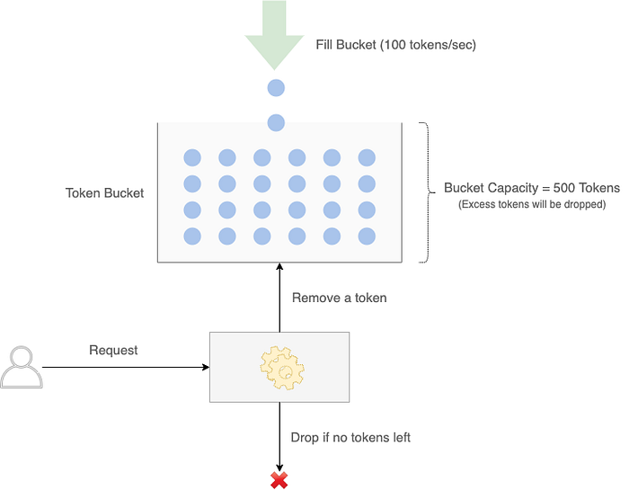
Token bucket can be implemented either by using a separate process to replenish the token or without one. Let’s assume:

rate = 100 tokens per minute, capacity = 500

Token Bucket Using a Separate Replenishment Process

In this, we have a single Redis key per user, which keeps track of the number of tokens available in the bucket for that user. A separate process adds 100 tokens to each user’s bucket (increment the value of the key by 100). No. of tokens for each user are capped at capacity.

When a request arrives, check the number of available tokens.

If tokens are available (value is > 0), allow the request and deduct one token (decrement the value by 1).
If tokens are not available, reject the request. All requests till the next replenishment cycle will be rejected.

Token Bucket Without a Separate Replenishment Process

Running a separate process for replenishing tokens is a big overhead. Also, it can be quite inefficient if you have a large no. of active users. Instead, we can use the approach described below.

Create a hash in Redis with user ID as key. The hash has two keys:

tokens: representing the number of tokens left
last_access: User’s last request timestamp

When we receive a request from a user, we do the following:

Fetch tokens and last_access for user
Replenish token bucket

NUM_TOKENS_TO_ADD = rate * delta, where delta = now - last access (difference in no. of seconds)
NEW_TOKEN_COUNT = tokens + NUM_TOKENS_TO_ADD
If NEW_TOKEN_COUNT > capacity, set NEW_TOKEN_COUNT = capacity (we can not have more than capacity tokens for any user)
Set tokens = NEW_TOKEN_COUNT

3. If tokens >= 1, allow the request and deduct a token. Else reject the request.

For this to work in a distributed setting, all the steps need to be implemented and executed using a Lua script so that all the steps run atomically.

A Simpler Token Bucket Approach (Without Burst)

A simpler variant of the token bucket algorithm, without the ability to burst, is suggested here. Again let’s assume 100 req/min:

When the first request arrives from a user, create a key for that user with value 100 and TTL of 1 min.
For every subsequent request, decrement the value.
If the value becomes zero, reject the request.
After 1 min from the initial request, the key will expire. For the next request, the key will be created again with a value of 100 and so on.

Generic Cell Rate Algorithm (GCRA)

GCRA is a sophisticated algorithm with a very low memory footprint. It allows for equal spacing between requests to reduce sudden load on servers. For example, if the rate limit is 10000 requests/hour, then GCRA makes sure that users can’t make all 10000 requests in a very short period of time (say a few seconds).

By default, requests will have to be equally spaced within a given interval. So for the above case, requests have to be spaced by 3600/10000 seconds or 360 ms. Any request made within 360 ms of the previous request will be rejected.

In order to avoid being too stringent on users, GCRA also allows for some bursts. If you specify a burst of 100, then users can make 100 requests in addition to their 1 req/360 ms. These 100 requests could be within a single 360 ms window or spaced across multiple windows.

To understand GCRA, we need to first look at the terminology used:

Let's say our rate limit is 100 req/second

period: Period for which rate limit is defined. In this case, 1 second or more accurately 1000 ms
rate: No. of requests allowed in period. In this case, it’s 100
emission_interval: Interval (or ideal spacing) between requests. It’s period/rate. In this case, it’s 10, which means ideally, requests should be emitted at 10ms intervals
burst: Max burst allowed
delay_tolerance: emission_interval * burst, if burst > 0. So, if burst is 5, then this is 50 ms
TAT: TAT is Theoretical Arrival Time i.e. the time when the next request is supposed to arrive as per the emission_interval. If burst is defined, delay_tolerance is also taken into account in TAT calculation

The essence of this algorithm is to calculate and store the TAT for the next request. If the next request arrives in the future w.r.t. it’s TAT, request is blocked. Otherwise, it’s allowed.

Let’s understand it using an example:

First Request

Let’s say the first user request arrives at 10:00:00.500 (Let’s call is ARRIVAL1).

TAT = ARRIVAL1 + emission_internal (Means ideally next request should arrive after 10ms i.e. at or after 10:00:00.510).

Allow request and store the TAT value for user in Redis.

Subsequent Requests

Without Burst

If we do not consider burst, then the algorithm is quite simple. We just need to check if the current request time is greater or less than the TAT i.e. whether the request arrives in future or past w.r.t. the TAT.

Let’s say the next request arrives at ARRIVAL2. Retrieve TAT from Redis.

If ARRIVAL2 < TAT, request arrives too soon. Reject.
If ARRIVAL2 >= TAT, request arrives on or after the allowed time. Allow. Also, update TAT as Max(ARRIVAL1, TAT) + emission_internal

The intuition behind this is quite simple. Requests should be spaced in time as the rate limit parameters. In the example we considered (100 requests/second), the spacing between requests must be at least 10 ms. If a request arrives within 10 ms of the previous request, it is rejected.

With Burst

The actual workload of a lot of applications is hardly ideal as described above. It’s usually bursty i.e. clients send a bunch of requests within a small time interval and then do not send any requests for some time. In such cases, GCRA can be overly stringent. For example, if a client sends 10 requests at the same time, only 1 will be allowed and 9 will be rejected.

Ideally, we would want to allow some burst in our rate limiting technique. The intuition behind burst in the context of GCRA is:

We start with a burst balance e.g. 5 (which is also the max burst)
burst balance dictates how many requests clients can send before TAT without being rejected
Each request sent before TAT consumes a unit from burst balance
Each request sent after TAT adds to the burst balance (up to the max burst). How much it adds depends on how long after the TAT it arrives.

To incorporate burst in the algorithm without complicating it (i.e. we just using a single variable TAT as before), we factor in a delay_tolerance and define a variable allowed_at, which is the time we look at to see whether the request should be allowed or rejected.

Without burst, allowed_at is same is TAT.

With burst, allowed_at = TAT - delay_tolerance

Again, let’s say the next request arrives at ARRIVAL2. Retrieve TAT from Redis.

allowed_at = TAT - delay_tolerance
If ARRIVAL2 < allowed_at, request arrives too soon. Reject.
If ARRIVAL2 >= allowed_at, Allow. Also, update TAT as Max(ARRIVAL1, TAT) + emission_internal

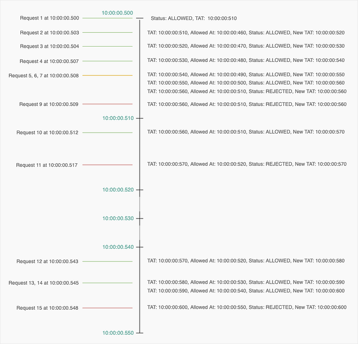
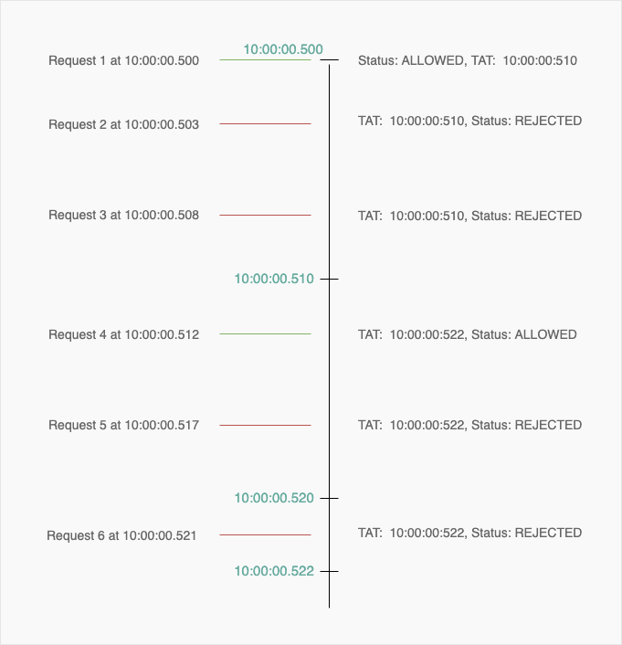
You can see burst (burst = 5) in action in the above diagram. We have allowed 5 additional requests than usual 1 in the first window. After that, further requests in that window are rejected. Since the entire burst balance has been consumed, it falls back to 1 request per interval. If the client doesn’t make any requests in the future interval (as in 10:00:00.520 - 10:00:00.530 and 10:00:00.530 - 10:00:00.540), it accumulates burst balance.

Here’s a sample implementation of GCRA in java:

// - Example rate limit is 100 requests/second with a burst of 5
long period = 1000L; // milliseconds
long rate = 100L;
long burst = 5;

long emissionInterval = period/rate;
long increment = emissionInterval;
long delayTolerance = emissionInterval * burst;

long arrival = System.currentTimeMillis(); // Time of the request

long TAT = getTAT(); // Get TAT from DB or cache
if (TAT == -1) {
    TAT = now;
}
else {
    TAT = Math.max(now, TAT);
}

long allowAt = TAT - delayTolerance;

if (arrival >= allowAt) {
  // Allow the request
  TAT = TAT + increment;
  storeTAT(); // Store TAT value in DB or cache
}
else {
  // Block the request
}

GCRA is used in the redis module redis-cell.

Rate Limiting Using Proxies

If you don’t want to implement rate-limiting yourself, you can use a proxy to do it for you. Rate limiting can be done at multiple levels:

API Gateway (Kong, Traefik, Ambassador, AWS API Gateway, etc.)
Reverse Proxy (Nginx, HAProxy)
Sidecar (Envoy)

The technique employed for implementing rate limiting differs between these technologies. Here we describe one called leaky bucket.

Leaky Bucket

Similar to the token bucket, leaky bucket also has a bucket with a finite capacity for each client. However, instead of tokens, it is filled with requests from that client. Requests are taken out of the bucket and processed at a constant rate. If the rate at which requests arrive is greater than the rate at which requests are processed, the bucket will fill up and further requests will be dropped until there is space in the bucket.

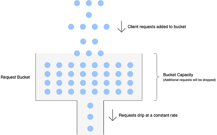
The bucket can be implemented as a FIFO queue. The size of the queue is equal to the bucket capacity. New requests are added to the queue and a separate thread can deque requests at a constant rate and send them for processing. If the queue is full, further requests are dropped until space becomes available.

There are more rate-limiting options available in different technologies. I would recommend reading the official documentation.

Running Multiple Instances of the Proxy
We need to be careful if we are running multiple instances of the proxy for high availability. Generally the rate limiting state is kept in the local memory and is not shared among instances. Check the official docs to see if there is support for distributed rate limiting.

Misc

In this article, we have not considered that there is some notion of cost associated with requests. We have assumed that each request is same as far as rate-limiting is concerned and each request consumes a single unit of the client’s allocated quota. If requests have an associated cost, the algorithms will need to be modified slightly to take the cost into account. In general, we can think of a request with cost N to be the same as N requests arriving at the same time.

References & Further Reading