Handling Overload With Concurrency Control And Load Shedding — Part 2

In the second part of this series, we are going to look at Netflix’s concurrency limits library and the algorithms it uses to implement adaptive concurrency control. As I also mentioned in the first article, this library is based on the TCP congestion control algorithms, which have been used for decades for congestion avoidance in TCP packet flow.

Before jumping on to the algorithms, I want to first provide some details about how this library integrates and works with our reference application described in the first article.

How Concurrency-limits Library Integrates With Spring Boot Applications

As we discussed previously, a Spring Boot application with a Tomcat web server has a fixed number of worker threads and there is a Tomcat queue for pending requests. Concurrency limits library integrates with the application using a servlet filter (A request interceptor can also be used). The servlet filter is used for pre and post-processing of the request.

The filter is a good place to track in-flight requests (IFR). During pre-processing, we can increment the IFR counter and then decrement it during post-processing. Note that the in-flight requests in this context are the requests that have been picked up by worker threads for processing. Requests waiting in the Tomcat queue do not count towards IFR. In fact, the Tomcat queue is not visible to the application.

The library tracks two variables:

• In-flight Requests (IFR): Number of requests that are currently being processed
• Concurrency Limit (CL): Current concurrency limit value

When a new request arrives, the IFR is checked against the concurrency limit.

• If IFR < CL, request is allowed and IFR is incremented by 1
• If IFR == CL, request is rejected

You can look at the code here.

Algorithms

Now that we have understood how concurrency limiting behavior looks like, let’s shift our focus to algorithms. The algorithms implemented in the concurrency limits library are inspired by TCP congestion control algorithms, which themselves are based on a feedback control system. Lets first define a few concepts:

System Output (Response Time)

For a feedback control system to work, we need to measure the system output which is then used in a feedback loop to tune system input. In our use case, the system output is the time it takes for the service to process requests, which is equivalent to Round Trip Time (RTT) used in TCP congestion control algorithms.

Adjustment Cycle

Adjustment cycle defines how often we adjust the concurrency limit value based on the system output (let’s call it Measured Response Time (MRT)). Adjustment cycle can be:

After Every Request
We can update the concurrency limit after every request, though it can make it very volatile. In this case, MRT will be the response time of that particular request.

Time-Based
We can use time-based windows e.g. every X seconds. The response times of all the requests in the window will be aggregated to compute the MRT. For aggregate, we can use average, median, or 90/95/99 percentile.

How large the time window should be, depends on the service. Large time windows may delay the overload detection and very small windows may make the concurrency limit volatile.

Count Based
This is same as above, but instead of time, we take a request count based window e.g. every X requests.

Desired System Output

The feedback control system also needs a desired system output which is compared against the measured system output to adjust the limits. In this case, the desired output is the response time we want the service to maintain (let’s call it Ideal Response Time(IRT)). How the IRT is defined depends on the algorithm used. Some algorithms require a fixed value e.g. 1 second. If the MRT goes above this value, the algorithm will start decreasing the concurrency until MRT < IRT. Other algorithms can automatically find IRT based on system’s steady state.

With the basic concepts defined, let’s take a look at the algorithms used by the concurrency limits library:

AIMD Algorithm

The Additive Increase/Multiplicative Decrease(AIMD) algorithm is inspired by the AIMD algorithm used for TCP congestion control. It uses the following parameters:

• initialConcurrency: Concurrency value to start with
• maxConcurrency: Maximum concurrency
• minConcurrency: Minimum concurrency
• timeout: When MRT reaches this value, the service is considered overloaded
• backoffRatio: Used to decrease concurrency when overload is detected. Its value is usually between 0.5 and 0.9

Concurrency Limit Adjustment

It works as follows:

• Start with an initial concurrency (initialConcurrency)
• Keep increasing the concurrency by adding 1 to the current concurrency value in every adjustment cycle (up to maxConcurrency or until overload is detected)
• As soon as overload is detected (i.e. MRT > timeout), back off (decrease concurrency) by multiplying current concurrency by backoffRatio (up to minConcurrency or until service is recovered from overload)

This will result in a chart like (with backoffRatio = 0.9):

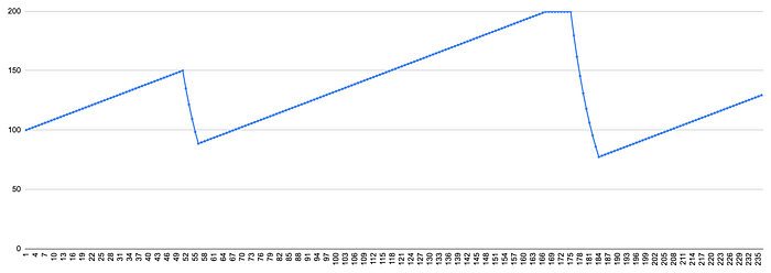
It starts with a concurrency of 100 and adds 1 to the concurrency in every update cycle. At 150, overload is detected and concurrency starts dropping by multiplying 0.9 at each step. At 90, the service recovers, and the additive increase cycle starts again. The concurrency reaches the maximum (200) and stays there until the service is overloaded again, after which it starts the multiplicative decrease cycle.

It keeps on going like this until it finds the right balance.

Vegas Algorithm

This again is based on the TCP Vegas algorithm for congestion control. It is different than AIMD in two significant ways:

• It does not require you to specify a reference system output value i.e. timeout. The algorithm computes this value dynamically.
• It tries to detect the overload conditions before the overload actually occurs and proactively takes necessary steps

Vegas uses a base MRT value i.e. the MRT value when service is working fine and not overloaded (let’s call it MRT_NoLoad) as a reference value to check whether any mitigation is required or not. MRT_NoLoad is computed as follows:

• Initially MRT_NoLoad is not set. In the first adjustment cycle, it is set to MRT.
• In subsequent adjustment cycles, it is updated to MRT if MRT < MRT_NoLoad i.e. MRT_NoLoad is the lowest MRT seen till now.
• Every X cycles, MRT_NoLoad is reset to the current MRT (irrespective of its value). This is called probing for new base MRT.

Concurrency Limit Adjustment

If the current MRT is greater than or equal to MRT_NoLoad, limit adjustment logic is triggered. Vegas uses the concept of a queue to estimate concurrency limits. The queue size is calculated as:

queueSize = currentConcurrencyLimit * (1 - MRT_NoLoad / MRT)
alpha     = 3 * Log10 (currentConcurrencyLimit)
beta      = 6 * Log10 (currentConcurrencyLimit)
threshold = Log10 (currentConcurrencyLimit)

To get some idea of these numbers, let’s take currentConcurrencyLimit as 100.

alpha     = 3 * 2 = 6
beta      = 6 * 2 = 12
threshold = 2

The algorithm considers the following scenarios:

No Queuing

It means the MRT is quite close to MRT_NoLoad. The library defines this condition as queueSize <= threshold.

To get some sense of it, with currentConcurrencyLimit as 100:

  MRT_NoLoad | MRT Limit 
 ------------|----------- 
         200 |       204 
         300 |       306

When there is no queuing, the service is doing quite well and we can aggressively increase the concurrency limit. The library uses the following:

newLimit = currentLimit + beta;

Manageable Queuing

It means the MRT has increased slightly, but it’s still not considered as overload. This condition is defined as threshold < queueSize < alpha.

  MRT_NoLoad | MRT Limit 
 ------------|----------- 
         200 |       212 
         300 |       319

If the queue size is manageable, we can still increase the concurrency limit, albeit by a smaller number.

newLimit = currentLimit + Log10 (currentLimit);

Excessive Queuing

The latencies have started to increase and this is the early sign of overload. We need to decrease concurrency limits to bring latencies down. This condition is defined as alpha <= queueSize < beta.

  MRT_NoLoad | MRT Limit 
 ------------|----------- 
         200 |       227 
         300 |       340

In this case, we decrease the concurrency limit as:

newLimit = currentLimit - Log10 (currentLimit);

Gradient Algorithm

The Gradient algorithm adjusts the concurrency limit by comparing the long-term and short-term response times. Like Vegas, it does not require you to specify a reference timeout value. The algorithm involves the following steps:

Measure Long Term Average MRT

The long-term average MRT is measured as the exponential moving average of MRTs in last N adjustment cycles. Let’s call it longMRT.

Compute Gradient

The gradient is computed using longMRT and current MRT (short-term MRT). We also need to define how much increase in MRT we are willing to tolerate (as compared to longMRT). If tolerance is 2, then short MRT can go up to twice the long MRT before we start reducing concurrency.

gradient = Max(0.5, Min(1.0, tolerance * longMRT / shortMRT));

The gradient will start with a value close to 1 and will remain there as long as shortMRT < tolerance * longMRT. If latencies start to increase, then shortMRT will increase, causing gradient to fall below 1.

Concurrency Limit Adjustment

The concurrency limit is adjusted using the gradient value and allowing for some queuing.

newLimit = gradient * currentLimit + queueSize;

queueSize can either be a fixed value (4 by default in the library) or could be a function of the current limit e.g. Log10 of the current limit.

The Gradient algorithm can be intuitively explained using various stages of the service.

Steady State

In this state, the service is doing well and MRTs are fairly stable. Gradient will be 1 causing the concurrency limit to increase by queueSize in every iteration. As concurrency is increased, it may increase the short MRT causing the gradient to fall, which in turn will lead to a drop in the concurrency limit. Overall, it’ll remain quite stable.

Steady State to Overload

If the service is experiencing overload, short MRT will keep increasing causing the gradient to shift towards a 0.5 value. This will in turn decrease the concurrency limit. If the load is sustained for a long period, the gradient and the limit will remain low, but longMRT will keep on increasing due to exponential moving average of higher short MRTs.

Overload to Steady State

When the service recovers, short MRTs will start decreasing, but the longMRT may take some time to go back to normal. It may be necessary to reduce longMRT outside of EMA if its value is very high. The library uses the following in every update cycle for this:

longMRT = longMRT * 0.95, if longMRT is more than twice the shortMRT

Next: In part 3 of the series, we explore some of the caveats with the concurrency limits library and discuss the alternative proxy-based approach.

Further Reading

• https://medium.com/@NetflixTechBlog/performance-under-load-3e6fa9a60581
• https://github.com/Netflix/concurrency-limits
• Goresilience: Concurrency limits library implemented in GO